Inventory Optimization Needs the Right Processes to Make a Difference

This article addresses the myths and truths about inventory optimization and why the right processes make all the difference.

We all dream of a perfect world
For supply chain managers charged with optimizing inventory, especially in the retail industry, Supply Chain Utopia might be a make-to-order environment where a customer walks into a store or visits a Web site to purchase a new shirt to go with a stylish summer outfit.

In a matter of minutes, a seamstress turns out a beautiful blue cotton shirt in just the right size. A few minutes later, the shirt is boxed in tissue paper and handed to the happy customer or dropped off at a parcel carrier for the last mile delivery.

In Supply Chain Utopia, retailers would always have ample capacity, raw materials, and labor to meet periods of average and peak demand. Inventory optimization would be taught in The History Of Supply Chain 101; inventory managers would bore their grandchildren with stories about distribution centers, stocking points, and back-of-the-store storage rooms from the good old days.

Related: 7 Principles of Supply Chain Management Redux

Unfortunately, Supply Chain Utopia is a myth. The truth of today’s competitive markets is that customers want instant purchase gratification while lead times for incoming merchandise can be 20 days to 180 days. That especially holds true for retailers at all stages of the transformation from single channels of business, such as a brick and mortar or catalog retailer, to multi- and omni-channel retailing from stores, catalogs, the Web, and other mediums. But, it also holds true for industrial distributors and manufacturers competing on a greater depth of product, drop shipments, and higher levels of customer service.

This does not mean we should stop developing demand-driven retail or distribution supply chain strategies with the concept of buy one and stock (replenish) one. In the meantime, however, most retailers and distributors will struggle to have the right SKU at the right place, in the right quantity, and at the right time to meet the demands of their customers.

To that end, many supply chain managers rely on expensive forecasting tools to optimize inventory across their networks. We believe there is another approach: By changing the flow of inventory from source to consumption through reduced cycle times, inventory positioning, and synchronizing supply chains based upon demand variability, managers can reduce their inventory levels without expensive forecasting tools, especially as the target fill rate increases.

At the least, optimizing inventory flow and positioning in combination with forecasting can deliver better results than relying on forecasting alone. In this article, we will highlight three retailers with varying levels of inventory challenges and the steps they took toward inventory optimization. In the process, we will call out many of the common myths and related truths on the subject of inventory optimization.

Forecasting and Inventory Positioning

Myth: Forecasting alone can solve the challenges that retailers face to service their customers.

Truth: Prior to implementing any forecasting solution, reduce the total cycle times and minimize variability between supply and demand points. Retailers and distributors alike require an optimal supply chain network, in combination with positioning inventory in the correct location.

Inventory is by far one of the largest components of working capital for most retailers and distributors. To meet mounting consumer expectations, both have attempted to solve inventory challenges by utilizing forecasting software to help determine what to buy and when to buy it. Retailers do need some level of forecasting due to the number of factors that affect their ability to time demand with supply and to allocate the right inventory—the right SKU—to the correct store location. We call that SKU LOC. As retailers expand, adding more store locations while increasing the number of SKUs they offer customers, the number of SKU LOC permutations increases.

To make the right allocations, forecasting solutions evaluate a number of variables, including supply lead time and variability, purchase order review periods, demand variability, lead times from the DC to the store, safety stock percentage, in-stock percentage, minimum presentation quantity, and shelf holding power. Each of these variables affects the amount of inventory in the supply chain. But which variable or combinations of variables has the greatest impact on inventory? How does dependent or independent demand variability affect inventory in combination with inventory positioning? And, how does a retailer avoid over-allocating or allocating to the wrong stores in order to minimize markdowns, lost gross margin, and transfers between stores?

Myth: Positioning inventory as far forward in a retailer’s supply chain (stores) is the optimal solution.

Truth: Over allocating inventory to stores increases markdowns, lost gross margin, and transfers between stores.

While some level of forecasting is required, forecasting alone won’t deliver all of the answers. Instead, retailers and distributors can enhance their ability to improve inventory turns, and reduce working capital while improving service, through careful inventory positioning, changing flow paths, and allocation strategies designed to improve the velocity of capital. Inventory positioning is not a new concept; however, few retailers and distributors utilize inventory positioning, multiple flow paths, and network design as a means to optimize inventory and improve service to their customers.

Let’s look at how three growing retailers, representing a variety of go-to-market strategies, optimized their inventory by reducing cycle times, inventory positioning, and synchronizing their supply chains based upon demand variability.

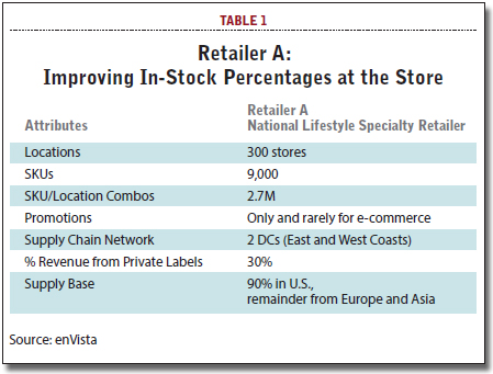
Retailer A is a national lifestyle and specialty retailer with 300 stores and 9,000 SKUs. Its stores are served from two DCs. A Pennsylvania DC serves the East Coast while the second facility in Utah serves the western half of the country. It rarely runs promotions and those are primarily aimed at its e-commerce customers. The heaviest traffic occurs on the weekends, with Friday, Saturday, and Sunday accounting for 57 percent of the retailer’s sales. Ninety percent of its supply base is located in the U.S., with a small percentage located in Europe and Asia. A third of its revenue comes from private-labeled merchandise. (See Table 1.)

Retailer A was challenged by a number of supply and demand variables. Each store carries the full 9,000 SKUs; however, stocking volume levels vary according to the size of the store, its geographic location, and its revenue. In all, there are 2.7 million possible SKU LOC combinations for allocating inventory. Demand for anyone SKU is relatively light compared to fast-moving CPG products: A high volume SKU sells just one unit every three weeks, and a typical product lifecycle lasts over a year. Once a new SKU is introduced to the market and allocated to the stores, 100 percent of the new SKU is placed on replenishment.

Prior to an optimization initiative, the inventory flow through the network resembled a pure distributor, not a retailer. The retailer did not pre-allocate inventory prior to receipt. Instead, new receipts were allocated evenly between stores, which were treated equally, no matter where they were located or regardless of the demand for an SKU in that store. When an SKU was received in a distribution center, it was put away into storage before it was allocated, picked, packed, and shipped to a store. Each store received only one shipment per week with the exception of stores in New York City, Los Angeles, and San Francisco. Purchase orders were reviewed once a month for 250 vendors.

The retailer’s biggest challenge was lost sales due to out of stocks. Its in-stock position was less than 91 percent at the store and less than 70 percent at the DC. An item that was out of stock at the store was even more likely to be out of stock at the DC, meaning little chance of replenishment.

Synchronizing Supply With Demand
Retailer A had one goal: Improve in-stock percentage to the store.

Retailer A’s number one goal was to synchronize supply with demand to decrease its out of stock position at the shelf. Doing so would improve sales, reduce the amount of safety stock maintained in the back room, and reduce the labor associated with cycle counting and replenishing the shelves. It achieved this through three steps.

Truth: Increasing purchase order frequency will improve the flow of inventory from supplier to DC, resulting in improved fill percentage and downstream distribution center in-stock percentage. The consequence is increased inbound transportation.

1) At the start of this project, the average supplier’s fill rate was 84 percent. This was partially due to the fact that suppliers received purchase orders in the third week of the month and were expected to ship an order during the first week of the next month. Many suppliers were not in a position to fulfill 100 percent of the order in weeks three and four. To address this imbalance, Retailer A increased its purchase order frequency from once a month to weekly for high volume suppliers, and to twice a month for the remaining vendors. By moving to weekly and bi-weekly re-ordering, the fill rate increased from 84 percent to 93 percent. Increased purchase order frequency directly increased the distribution center in-stock percentage from 70 percent to 88 percent.

Truth: Increasing order delivery frequency reduces cycle time from DC to store, improving the flow of inventory and in-stock percentage. The consequence is increased outbound transportation.

2) Retailer A also increased its order frequency by volume group to reduce the average replenishment cycle time from nine days to five and a half days. That allowed 65 percent of the stores to sell a unit over the weekend and have a replacement on the shelf by the next Friday, in time for busy weekend traffic. Retailer A’s in-stock percentage improved from 91 percent to 96.3 percent, improving comparable sales by 2 percent. The retailer reduced operational payroll by $2.9 million by improving its shipment to shelf percentage from 55 percent to 94 percent. That eliminated the need to maintain safety stock in the back stock rooms and the need to allocate labor to cycle count extra inventory that was not required.

Truth: Retailers must align and design inventory flow paths to match seasonal and promotional demands - by doing so, they reduce cycle time and improve speed to market.

3) Prior to this project, Retailer A had a 100 percent post allocation inventory strategy: All new receipts were received and put away into storage before they were allocated, picked, packed, and shipped via LTL carriers. However, as a result of analyzing inventory flow, Retailer A realized that the demand for some SKUs was predictable. That led to a new model, where 15 percent of SKUs were pre-allocated - or put-to-stores. Newly received inventory was processed at receiving and flowed through the facility to a parcel carrier. On average, Retailer A reduced four days of cycle time for new SKUs by utilizing a put-to-store distribution flow and a change in carrier modes. In addition, Retailer A reduced DC labor by utilizing the pre-allocation put-to-store process. The change in allocation strategy and carrier mode allowed Retailer A to be the first to market with its fashion-oriented merchandise, driving improved sales.

When the initiative was complete, Retailer A optimized inventory by increasing the velocity of inventory through the supply chain. It is important to note that the retailer made no changes to its physical distribution locations. Rather, it focused on synchronizing inventory flow based upon demand patterns. This was accomplished by reducing cycle time from suppliers, increasing purchase order frequency, and reducing cycle time in its DCs and the cycle time from DC to Store. In-stock percentages and comparable sales increased while safety stock inventory levels decreased.

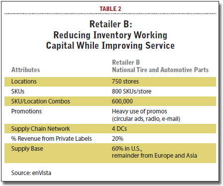
Retailer B is a national tire and automotive parts chain. It stocks 800 SKUs in each of its 750 stores. That creates 600,000 possible STORE LOC permutations when it comes to allocating inventory. Like many tire and parts retailers, it uses radio, e-mail, and newspaper circular ads to promote sales.

Twenty percent of its revenue comes from private label products. Prior to an inventory optimization project, it operated a network of four distribution centers; 60 percent of its supply base is domestic with the remainder coming from Europe and Asia. (See Table 2.)

A number of factors impeded Retailer B’s ability to optimize inventory. Beyond market constraints related to the industry, it was hampered with a demand pattern called “intermittent demand,” or “sporadic demand.” (See Exhibit 1.)

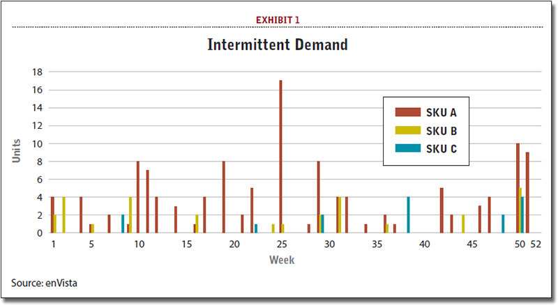
Intermittent demands patterns occur with slow-moving items that are purchased infrequently and in variable quantities. An item purchased this month may not be purchased again for another three months. Plotted on a chart, intermittent demand will have a number of zero demand periods. Yet, to meet customer demand, the retailer must always keep some level of inventory in stock.

Determining the right stocking level for SKUs with intermittent demand is difficult with traditional forecasting techniques because conventional technologies look for predictable demand patterns with trends or seasonality. Intermittent demand, however, is characterized by the number of zero demand periods that are not easy to predict. When a traditional forecasting tool sees those periods of zero demand, it assumes there must be an error. That results in inaccurate forecasts and either stockouts or too much inventory.

Myth: Extra inventory equals better service. In many cases, it can negatively affect sales by over-allocating inventory to the wrong store.

With 800 tire SKUs and 750 locations, equating to 600,000 SKU and location combinations, the ability to accurately forecast at the store level became very difficult. In order to meet forecasted consumer demand, the retailer overstocked inventory at all stores (cycle and safety stock). This was compounded by the fact that the retailer replenished the stores just once a week, regardless of store volume. The existing inventory management approach created less than desirable store inventory turns and increased working capital to manage the retailer’s intermittent demand patterns.

Excess inventory was also an issue at the four DCs. In addition to stocking excess inventory at the stores to cover demand variability, the retailer was stocking at the DCs to compensate for supply variability. Excess inventory across the supply chain was compounded by the fact that the retailer was making forward buying decisions to protect it from pricing volatility by its supply base:

Retailer B had one goal: Reduce inventory working capital in its supply chain, while improving service.

To reduce its investment in inventory at both the stores and the DC’s while dealing with intermittent demand, Retailer B took several steps, including a redesign of its supply chain network.

1) Retailer B’s first step was to evaluate its supply chain network while simultaneously evaluating demand patterns. Retailer B moved from a four DC, single-tiered network strategy to a multi-echelon tiered network that included two cross-dock facilities and 31 spoke locations. (See Exhibit 2.)

The change to the physical distribution network allowed the retailer to improve forecasting accuracy by aggregating store-level demand from 750 locations to 31 distribution locations (spokes). That allowed the retailer to reduce safety stock in the stores by 20 percent.

Like Retailer A, Retailer B increased its order delivery frequency from one time to five times per week for many store locations. The ability to sell an SKU and have it available on the shelf within 24 hours (leveraging a pull system) allowed the retailer to reduce inventory in the stores.

Truth: An optimal supply chain network design, in combination with inventory flow path analysis, will reduce inventory working capital. It is very important when evaluating intermittent demand patterns to look at demand patterns by store and not the aggregate demand patterns for all stores.

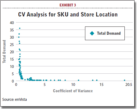
2) The retailer determined the coefficient of variance (CV) for each SKU and store location combination (Exhibit 3).

The CV analysis determined the unique physical distribution flows for each item, and defined which SKU LOCs required inventory forward in the supply chain (store or spoke) and which SKUs could be moved back in the supply chain (spoke and DC). By positioning inventory closer to where it was in demand, while increasing store shipment frequency, the retailer witnessed a 4.15 percent to 9.72 percent increase in comparative sales, compared to the non-test stores in the same geography.

Truth: CV analysis is used to help determine inventory flow paths (push vs. pull) and inventory positioning. Each SKU, or category of SKUs, requires unique physical distribution flows in order to optimize inventory and improve service levels.

3) Retailer B utilized economic order quantities for each item at all of the stores. With the introduction of hubs and spokes in the network, inventory that was less frequently demanded could now be held at the DC, shipped to the spokes, and then pulled from the spokes to the stores when a purchase was made, versus pushing and cross-docking tires with a low CV (Exhibit 4).

The economic order quantities were adjusted by product-location combination because every item demand varied from store to store. This solution increased inventory turns at the stores by 60 percent and contributed to a one-time working capital reduction of $24.6 million, as well as reducing annual carrying costs by $35.9 million over a period of five years.

Truth: First optimize inventory flows paths based upon supply and demand variability, and then develop your physical distribution and transportation network.

Retailer C operates 350 general merchandise and pharmacy locations, stocking as many as 25,000 SKUs per store. That equates to 8.75 million possible SKU LOCs across the chain. In addition to relying heavily on newspaper circular ads and radio and television promotions, the retailer recently developed an e-commerce strategy to promote sales. Less than 10 percent of its revenue is derived from sales of private-label merchandise. (See Table 3.)

It operated an extensive network of regional DCs, managing inventory from a supply base that is primarily located in the U.S., with 20 percent of its suppliers located in Asia.

Retailer C was challenged by multiple store formats, a very large SKU assortment, slow inventory turns, and physical distribution constraints that forced it to push inventory out to the stores - 100 percent of its inventory was pre-
allocated before it was received at a DC.

As a result, a lot of emphases was placed on improving forecast accuracy and allocating the correct inventory to the correct store. The retailer sourced the majority of its general merchandise from domestic suppliers with a 25 day average lead time from the time of purchase to the time the product was delivered to a flow-through DC. The retailer utilized a rolling six-week forecast and evaluated buys by category on a bi-weekly and monthly basis. Large volume stores were replenished twice a week while smaller stores received a weekly replenishment. Company-wide, inventory turns were less than three times a year.

By pushing inventory out to the stores, Retailer C generally sported an in-stock percentage of nearly 98 percent. The challenge with a 100 percent pre-allocation, or push, inventory flow model was that if the forecast was incorrect at the time inventory was pushed to the store, there was no room on the shelves. While the in-stock percentage looked good on the shelf, inventory piled up in a back stock room, which required additional store operational labor to receive, put away, replenish, and cycle count.

Retailer C had one goal: Develop a demand-driven supply chain.

With inventory turns at less than three times per year and back stock rooms overflowing with inventory, Retailer C took steps to synchronize its supply with demand and develop a demand-driven supply chain.

1) Retailer C’s physical distribution network consisted of four regional DCs, geographically located to manage and optimize transportation costs. However, the DCs were designed as 100 percent flow-through distribution centers—they had no reserve storage areas to hold buffer inventory. Like Retailer B, Retailer C completed a CV analysis to understand the demand variability by SKU and product category. The CVs for over 30,000 SKUs were greater than a 2.0 value.

That meant the SKUs had a tremendous amount of variability within the season and post-season. Inventory management was also challenged because Retailer C is highly promotional, but most inventory has a six-week lead time. That required moving the retailer’s inventory closer to its demand points.

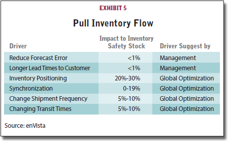
This necessitated a change from a 100 percent flow-through model to 20 percent flow-through and 80 percent pull. The physical layouts of the retailer’s facilities had to be changed to support a pull inventory flow (Exhibit 5).

Truth: Inventory positioning has the largest impact on optimizing inventory for retailers and distributors.

2) Retailer C’s leadership realized that if they wanted to reduce company-wide inventory, they needed to evaluate their store planogram and visual merchandising strategy. Retailer C looked at SKUs that were double and triple-faced and determined the correlation between excess inventory and their planogram strategy. By reducing SKU faces, Retailer C could reduce excess inventory (safety stock), which allowed the retailer to increase its assortment without increasing its inventory investment. The retailer could now add 10,000 additional SKUs (increasing the size of the assortment). The exercise revealed that the retailer’s visual merchandise strategy (depth of shelves), store planograms, and minimum presentation quantities had a negative impact on inventory working capital.

Truth: Space optimization, SKU assortments, and inventory flows must be aligned in order to reduce total inventory in the supply chain.

3) By involving cross-functional groups and completing detailed Value Stream Maps, the merchants, buyers, allocators, distribution, transportation, and finance functional teams understood how lead time, supply time, and supply and demand variability affected overall inventory performance. By mapping decision points, systems configuration, and system policies, Retailer C determined that processes and their supporting systems were not aligned. For example, all stores’ lead times from DC to the stores were set to the longest lead time—seven days—while many stores’ lead times were less than three days. This equated to four to five extra days of safety stock. In fact, Retailer C’s replenishment system actually supported lead time from DC to store but had not been configured to reflect the actual lead time.

Truth: Functions within organizations become silos, however, items and inventory cut across organizations horizontally. It is important that all functional teams understand the flow of inventory and how the decisions they make affect inventory performance.

No Silver Bullet
Looking over these three examples, it is clear there is no silver bullet that will optimize a retailer’s or distributor’s inventory - no one truth - including costly forecasting systems.

However, there are methods and processes that retailers and distributors can use to develop and ensure a demand-driven supply chain.

Inventory optimization is a derivative of a sound supply chain process design, controls, and measurements. Inventory is decreased by reducing lead times, inventory positioning, and synchronizing supply and demand order and delivery frequencies to meet the needs of customers.

The starting point is often with simple inventory flows and value stream maps across the supply chain.

About the Author

Jim Barnes is the President and CEO of enVista, a supply chain consulting and IT services firm. He has spent 22 years deploying supply chain solutions and synchronizing material and information flow for Fortune 500 companies. He can be reached at [email protected]. For more information, visit enVista on SC24/7.

More SC24/7 content on “Inventory Optimization”